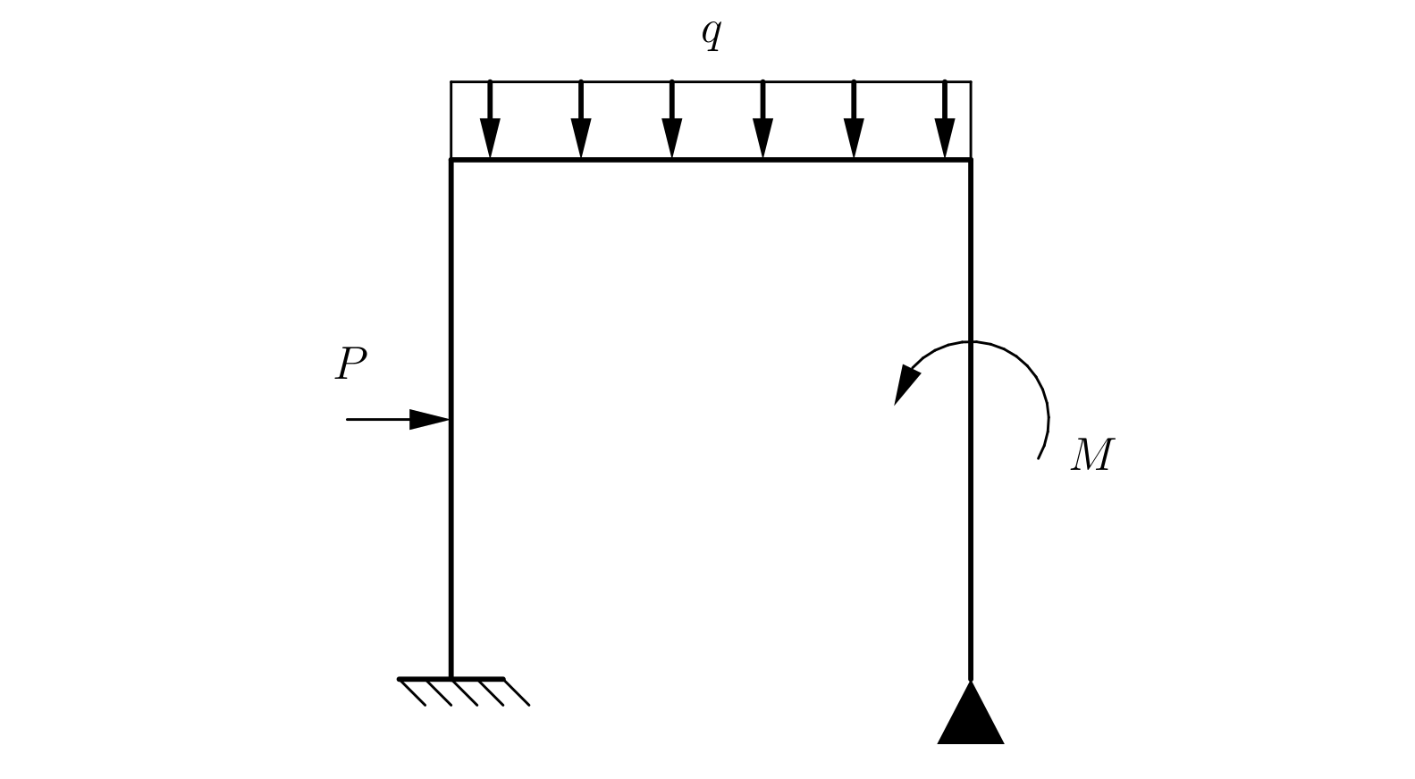
Consider a planar frame that is discretized into finite elements.

A frame structure carries axial forces, shear forces, and bending moments. The loading may be either distributed or concentrated.

Frame Discretization

The density and type of discretization depend on the geometry, loading conditions, and material properties.

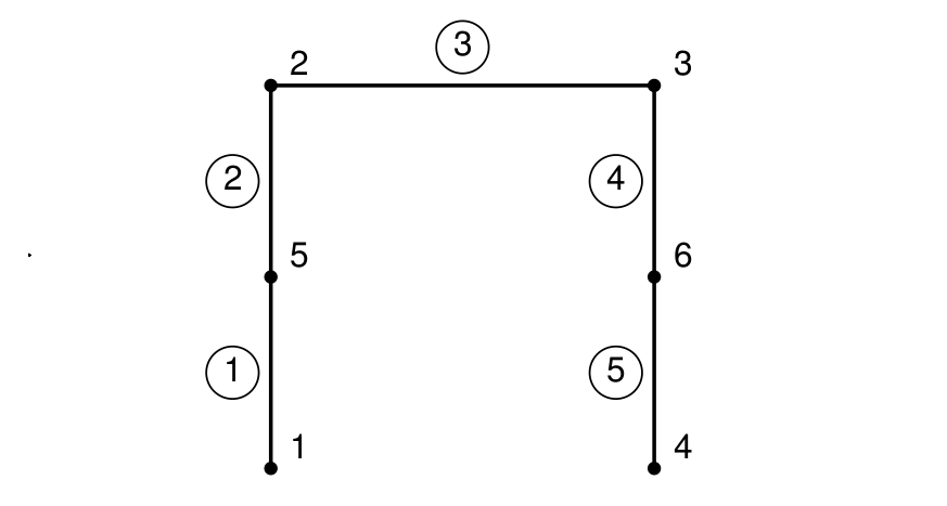
Each node has three degrees of freedom.

Governing Equations of the Frame Finite Element

A frame finite element is a combination of:
• a truss (bar) element with stiffness $EA$ subjected to distributed axial load $q^p$,
• a beam element with stiffness $EI$ subjected to distributed transverse load $q^b$.

At each node, there are three generalized nodal displacements and the corresponding generalized nodal forces. These quantities can be expressed in both local and global coordinate systems.

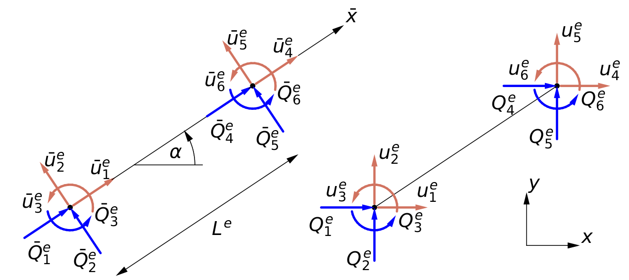
Local and global coordinate systems.

Let us recall the stiffness matrices for a bar and a beam element. We introduce subscripts to distinguish them:
• subscript $_p$ denotes the bar element,
• $_b$ denotes the beam element.

$$\k_p = \frac{EA}{L} \begin{bmatrix} 1 & -1 \\ -1 & 1 \end{bmatrix} \qquad \boldsymbol{k}_b = \frac{2EI}{L^3} \begin{bmatrix} 6 & 3L & -6 & 3L\\ 3L & 2L^2 & -3L & L^2\\ -6 & -3L & 6 & -3L\\ 3L & L^2 & -3L & 2L^2 \end{bmatrix}$$

By combining these two matrices, we obtain the local stiffness matrix of the frame element:

$$\bar{\boldsymbol{k}}= \frac{EA}{L} \begin{bmatrix} 1 & 0 & 0 & -1 & 0 & 0\\ 0 & 0 & 0 & 0 & 0 & 0\\ 0 & 0 & 0 & 0 & 0 & 0\\ -1 & 0 & 0 & 1 & 0 & 0\\ 0 & 0 & 0 & 0 & 0 & 0\\ 0 & 0 & 0 & 0 & 0 & 0 \end{bmatrix} + \frac{2EI}{L^3} \begin{bmatrix} 0 & 0 & 0 & 0 & 0 & 0\\ 0 & 6 & 3L & 0 & -6 & 3L\\ 0 & 3L & 2L^2 & 0 & -3L & L^2\\ 0 & 0 & 0 & 0 & 0 & 0\\ 0 & -6 & -3L & 0 & 6 & -3L\\ 0 & 3L & L^2 & 0 & -3L & 2L^2 \end{bmatrix}$$

In an analogous way, the local vector of external loads is obtained as the sum of the bar and beam contributions. The distributed load vectors for the bar and beam elements are:

$$\mathbf{f}_p = \frac{1}{2} q^p L \begin{bmatrix} 1 \\ 1 \end{bmatrix}, \quad \mathbf{f}_b = \frac{q^b L}{12} \begin{bmatrix} 6 \\ L \\ 6 \\ - L \end{bmatrix}$$

To combine them, they must be expressed in a common coordinate system. Additionally, we rename the distributed loads:

$$\bar{\mathbf{f}} = \frac{q^P L}{2} \begin{bmatrix} 1\\0\\0\\1\\0\\0 \end{bmatrix} + \frac{q^B L}{12} \begin{bmatrix} 0\\6\\L\\0\\6\\-L \end{bmatrix}$$

The same procedure applies to the nodal force vector. Therefore, the equilibrium equation for the frame element in the local coordinate system can be written as:

$$\bar{\boldsymbol{k}} \, \bar{\mathbf{u}} = \bar{\mathbf{f}} + \bar{\mathbf{Q}}$$

To express this equation in the global coordinate system, a transformation is required:

$$\mathbf{T} = \begin{bmatrix} \mathbf{t} & \mathbf{0} & \mathbf{0} \\ \mathbf{0} & 1 & \mathbf{0} \\ \mathbf{0} & \mathbf{0} & \mathbf{t} \end{bmatrix}, \quad \mathbf{t} = \begin{bmatrix} \cos\alpha & \sin\alpha \\ -\sin\alpha & \cos\alpha \end{bmatrix}$$

The angle $\alpha$ is the (positive) rotation angle defining the transformation.

Applying the transformation rules, the stiffness matrix in global coordinates becomes:

$$\boldsymbol{k} = \mathbf{T}^T \bar{\boldsymbol{k}} \mathbf{T}$$

Similarly, for the nodal force vector, displacement vector, and distributed load vector:

$$\mathbf{f} = \mathbf{T}^T \bar{\mathbf{f}}, \quad \mathbf{Q} = \mathbf{T}^T \bar{\mathbf{Q}}, \quad \mathbf{u} = \mathbf{T}^T \bar{\mathbf{u}}$$

After performing these transformations, the final equation in the global system is:

$$\boldsymbol{k} \mathbf{u} = \mathbf{f} + \mathbf{Q}$$