Introduction

In many engineering problems, the geometry of the structure and the nature of the loading allow the three-dimensional problem to be simplified into a two-dimensional one. Such simplifications are extremely important in computational mechanics, since they significantly reduce the computational cost while still providing sufficiently accurate results for many practical applications.

Typical examples of structures modeled using two-dimensional assumptions include:
• thin steel plates,
• bridge deck slabs,
• retaining walls,
• concrete dams,
• tunnels,
• long embankments and soil structures.

Depending on the geometry and loading conditions, two main idealizations are commonly used:
• plane stress,
• plane strain.

Plane stress

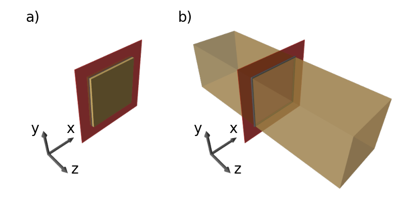
The plane stress condition occurs in thin structural elements such as plates or sheets loaded within their plane. It is assumed that the stress components perpendicular to the plane are negligibly small

$$\sigma_{33} = \sigma_{13} = \sigma_{23} = 0.$$

However, this does not mean that the corresponding strain components are equal to zero. In particular, the strain component $\varepsilon_{33}$ results from the Poisson effect.

Plane strain

The plane strain condition occurs in structures that are very long in one direction, where both geometry and loading do not vary along the z-coordinate. In this case, the strain components perpendicular to the analyzed plane are assumed to vanish

$$\varepsilon_{33} = \varepsilon_{13} = \varepsilon_{23} = 0.$$

In contrast to the plane stress condition, the stress component $\sigma_{33}$ is generally nonzero and results from the constraint of deformation in the 3-direction.

Stress and Strain State

For both assumptions, the in-plane stress and strain state is described by the following vectors

$$\boldsymbol{\sigma}=\begin{bmatrix}\sigma_x \\\sigma_y \\\sigma_{12}\end{bmatrix}, \qquad\boldsymbol{\varepsilon}=\begin{bmatrix}\varepsilon_{11} \\\varepsilon_{22} \\\gamma_{12}\end{bmatrix}$$

After reduction of the three-dimensional Hooke’s law, the constitutive equation takes the form

$$\boldsymbol{\sigma}= \mathbf{D}\, \boldsymbol{\varepsilon},$$

For the plane stress condition, the material stiffness matrix is given by

For the plane strain condition, the stiffness matrix becomes

$$\D = \cfrac{E}{(1+\nu)(1-2\nu)}\mat{1-\nu}{\nu}{0}{\nu}{1-\nu}{0}{0}{0}{\cfrac{1-2\nu}{2}}$$

It should be emphasized that both matrices are derived directly from the three-dimensional constitutive equations for isotropic linear elasticity by introducing the appropriate kinematic assumptions for plane stress or plane strain conditions.

Using the three-dimensional Hooke’s law, the out-of-plane strain and stress components can be computed as

• for plane stress

$$\varepsilon_{33}= -\frac{\nu}{E}\left(\sigma_{11}+\sigma_{22}\right)$$

• for plane strain

$$\sigma_{33}=\nu\left(\sigma_{11}+\sigma_{22}\right)$$

Discretization

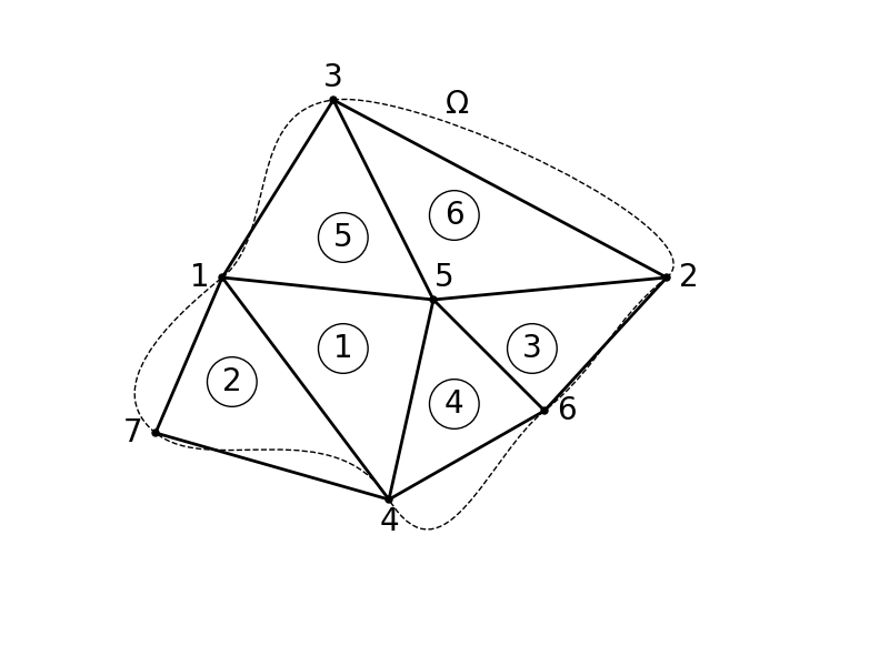
In the finite element method, the continuous two-dimensional domain is replaced by a finite number of smaller subdomains called finite elements. This process is referred to as discretization or meshing. The collection of all elements is called the finite element mesh. For two-dimensional problems, the computational domain is discretized using planar elements.
The most commonly used element types are:

• triangular elements,
• quadrilateral elements.

The geometry of the structure may be represented inaccurately if the number of finite elements is too small, especially in regions with highly curved boundaries or strong geometric variations. For this reason, mesh refinement is often required near curved edges, holes, supports, or regions where high stress gradients are expected.

Each finite element is connected to neighboring elements through nodes.
The unknown field variables, such as displacements, are computed at the nodes and interpolated inside the element using appropriate shape functions.

For two-dimensional structural problems under plane stress or plane strain assumptions, each node possesses two translational degrees of freedom.

Meshing algorithms

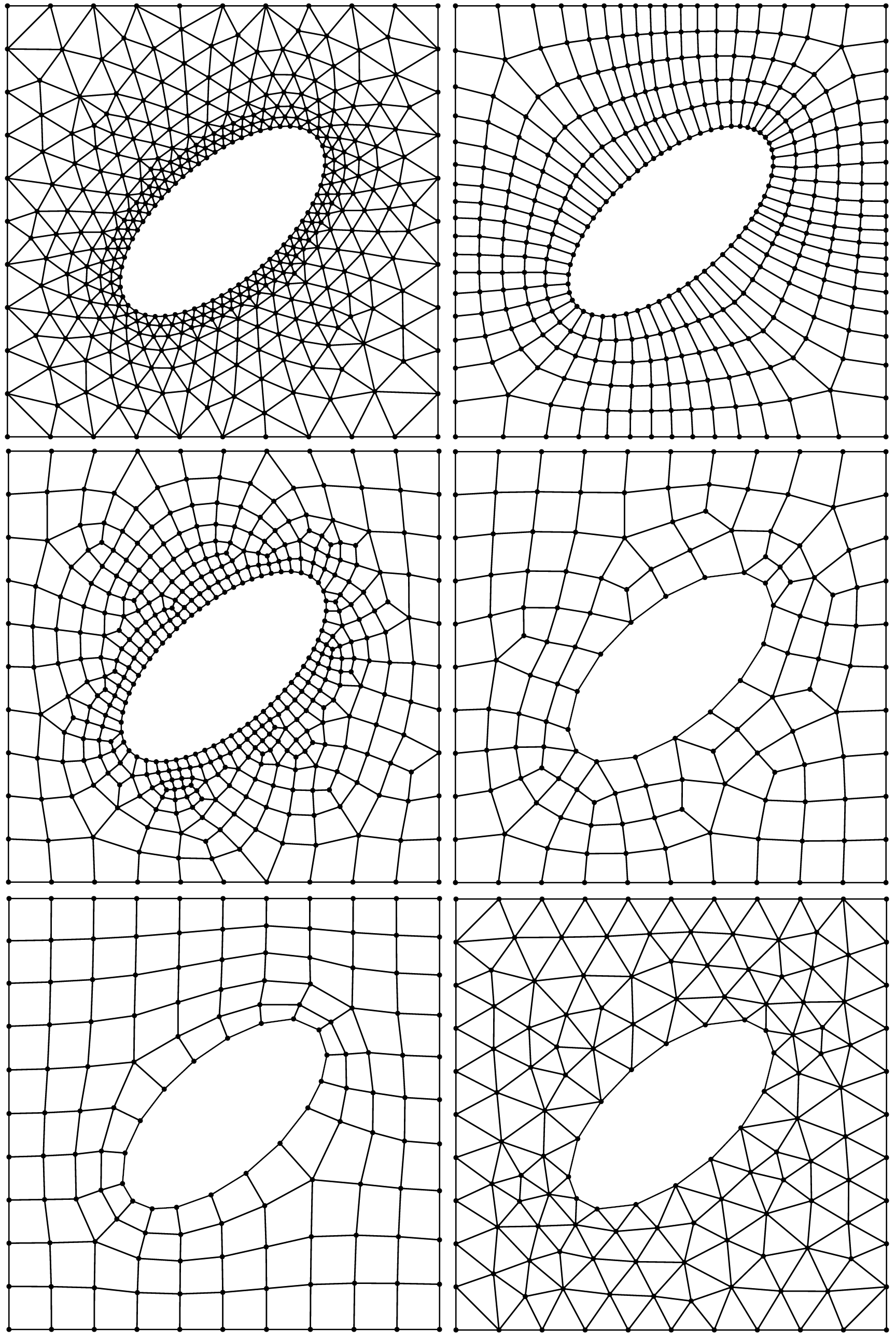
Modern finite element software provides many different meshing algorithms capable of generating meshes automatically for complex geometries. The choice of the meshing algorithm and element type has a significant influence on the quality of the numerical solution, computational efficiency, and the ability to accurately represent the geometry of the analyzed structure.

For two-dimensional problems, meshes may be generated using structured or unstructured approaches.
Structured meshes are usually composed of regular quadrilateral elements and provide high numerical accuracy for simple geometries. Unstructured meshes are typically based on triangular elements and are better suited for complicated geometries with curved boundaries or holes.

Commonly used meshing techniques include:
• Delaunay triangulation,
• advancing front methods,
• mapped meshing,
• quadtree-based algorithms.

Different meshing algorithms may produce significantly different element distributions even for the same geometry. On the figure below, several meshes generated using different element types and meshing strategies are presented.

In practical finite element analysis, the mesh should satisfy several important requirements:
• elements should have regular shapes and avoid excessive distortion,
• the mesh should be refined in regions with large stress gradients,
• element sizes should vary smoothly throughout the domain,
• the geometry of curved boundaries should be accurately approximated.

Poor mesh quality may lead to inaccurate stress predictions, slow convergence, or numerical instabilities.
For this reason, mesh generation is considered one of the most important stages of the finite element modeling process.

Finite element formulation

For two-dimensional elasticity problems under plane stress or plane strain assumptions, the displacement vector contains only two components

$$\mathbf{u} =\begin{bmatrix}u \\v\end{bmatrix}$$

where $u$ and $v$ denote the displacement components in the \(x\)- and \(y\)-directions, respectively.

The strain vector is defined as

$$\boldsymbol{\varepsilon} = \begin{bmatrix} \varepsilon_{11} \\ \varepsilon_{22} \\ \gamma_{12} \end{bmatrix} = \begin{bmatrix} \dfrac{\partial u}{\partial x} \\ \dfrac{\partial v}{\partial y} \\ \dfrac{\partial u}{\partial y} + \dfrac{\partial v}{\partial x} \end{bmatrix},$$

while the stress vector takes the form

$$\boldsymbol{\sigma} = \begin{bmatrix} \sigma_{11} \\ \sigma_{22} \\ \sigma_{12} \end{bmatrix}$$

The finite element stiffness matrix is obtained from the principle of virtual work.
Assuming constant thickness over the element domain, the element stiffness matrix may be written as

$$\mathbf{k}= h \int_A \mathbf{B}^T \mathbf{D} \mathbf{B} \; dA$$

where:
• $A$ - element area,
• $h$ - element thickness,
• $\D$ - constitutive matrix,
• $\B$ - strain-displacement matrix.

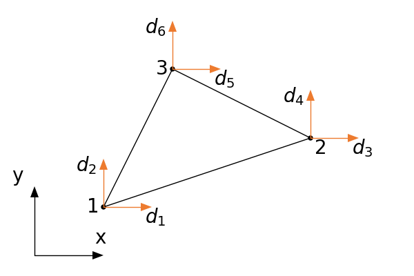
Three-Node Constant Strain Triangle (CST)

One of the simplest two-dimensional finite elements is the three-node triangular element, commonly referred to as the Constant Strain Triangle (CST) element. The element consists of three corner nodes connected by straight edges.

The displacement field inside the element is approximated using linear Lagrange interpolation

$$\mathbf{u} =\mathbf{N}\mathbf{d},$$

where

$$u(x,y)=\sum_{i=1}^{3}N_i(x,y)u_i,\qquad v(x,y)=\sum_{i=1}^{3}N_i(x,y)v_i.$$

The nodal displacement vector is given by

$$\mathbf{d} = \begin{bmatrix} u_1 & v_1 & u_2 & v_2 & u_3 & v_3 \end{bmatrix}^{T}$$

The shape functions are assembled into the interpolation matrix

$$\mathbf{N}^e = \begin{bmatrix} N_1 & 0 & N_2 & 0 & N_3 & 0\\ 0 & N_1 & 0 & N_2 & 0 & N_3 \end{bmatrix}.$$

Since the approximation is linear, the displacement field may also be written as

$$u = c_1 + c_2x + c_3y,\qquad v = c_4 + c_5x + c_6y.$$

The linear triangular shape functions are defined as

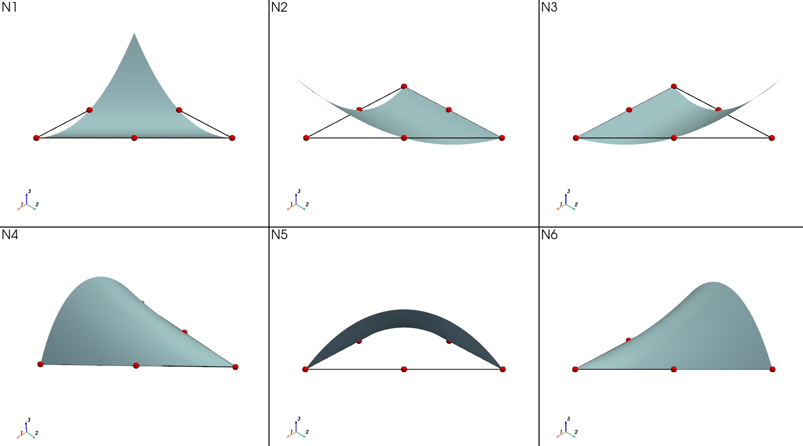
$$\begin{aligned} N_1 &= \frac{1}{2A} \left[ x_2y_3-x_3y_2 + (y_2-y_3)x + (x_3-x_2)y \right], \\ N_2 &= \frac{1}{2A} \left[ x_3y_1-x_1y_3 + (y_3-y_1)x + (x_1-x_3)y \right], \\ N_3 &= \frac{1}{2A} \left[ x_1y_2-x_2y_1 + (y_1-y_2)x + (x_2-x_1)y \right]. \end{aligned}$$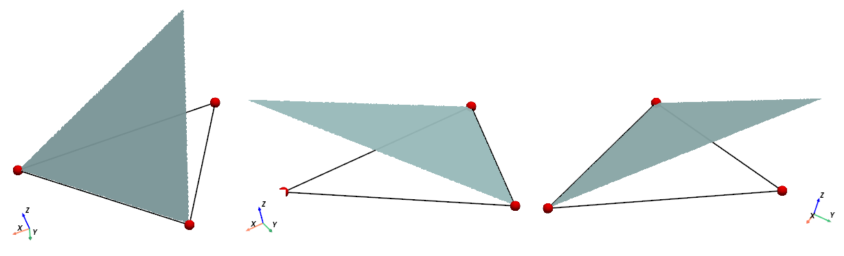

The strain field is computed using the differential operator matrix

$$\mathbf{L}= \begin{bmatrix} \dfrac{\partial}{\partial x} & 0\\ 0 & \dfrac{\partial}{\partial y}\\ \dfrac{\partial}{\partial y} & \dfrac{\partial}{\partial x} \end{bmatrix}.$$

The strain-displacement matrix is therefore

$$\mathbf{B}= \mathbf{L}\mathbf{N}= \frac{1}{2A^e} \begin{bmatrix} y_2-y_3 & 0 & y_3-y_1 & 0 & y_1-y_2 & 0\\ 0 & x_3-x_2 & 0 & x_1-x_3 & 0 & x_2-x_1\\ x_3-x_2 & y_2-y_3 & x_1-x_3 & y_3-y_1 & x_2-x_1 & y_1-y_2 \end{bmatrix}$$

The strain vector inside the element is obtained as

$$\boldsymbol{\varepsilon}=\mathbf{B}\mathbf{d}.$$

It can be observed that the matrix $\mathbf{B}$ does not depend on spatial coordinates $x$ and $y$.
Consequently, the strain field is constant throughout the element domain. For this reason, the element is called the Constant Strain Triangle (CST).

The CST element is computationally efficient and easy to implement, but it may produce poor accuracy when modeling bending-dominated problems or regions with large stress gradients.
Therefore, mesh refinement is often required when CST elements are used.

Six-Node Linear Strain Triangle (LST)

A more accurate triangular element frequently used in two-dimensional elasticity problems is the six-node triangular element, commonly referred to as the \textbf{Linear Strain Triangle (LST)} element.

In addition to the three corner nodes, the element contains three midside nodes located on each edge.
Each node possesses two translational degrees of freedom.

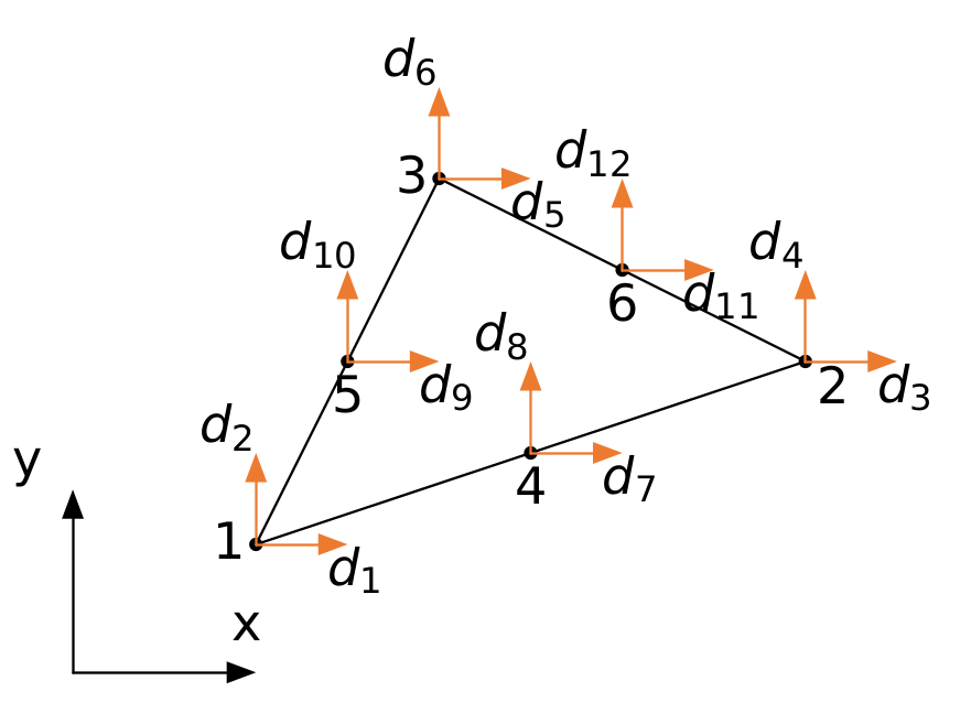
The nodal displacement vector is defined as

$$\mathbf{d}= \begin{bmatrix} u_1 & v_1 & u_2 & v_2 & u_3 & v_3 & u_4 & v_4 & u_5 & v_5 & u_6 & v_6 \end{bmatrix}^{T}$$

Unlike the CST element, the displacement field is approximated using quadratic interpolation functions.
The displacement components are therefore represented by second-order polynomials

$$u(x,y) =c_1 + c_2x + c_3y + c_4x^2 + c_5xy + c_6y^2,$$ $$v(x,y) = c_7 + c_8x + c_9y + c_{10}x^2 + c_{11}xy + c_{12}y^2.$$

Because quadratic interpolation is used, the strain field varies linearly inside the element domain.
This significantly improves accuracy compared to the CST element, especially for:
• bending-dominated problems,
• curved geometries,
• stress concentration regions.

The LST element provides smoother stress distributions and usually achieves higher accuracy with fewer elements than the CST formulation. However, the increased accuracy comes at the cost of higher computational effort due to the larger number of degrees of freedom and more complicated numerical integration.

For this reason, CST elements are often preferred for simple preliminary analyses, while LST elements are commonly used in practical engineering simulations requiring improved solution accuracy.